The Traveling Salesman Problem Is NP-Hard. EAX Matched the Optimum on 24,978 Cities.
November 22, 2026
Ask for the poster child of an impossible problem and you’ll get the Traveling Salesman Problem: given a set of cities and the distances between them, find the shortest loop that visits every city exactly once and returns home.
The reason it’s famous is arithmetic. With 60 cities on a symmetric map there are 59!/2 possible tours: about 7 × 10⁷⁹, a 7 followed by 79 zeros. That is in the same ballpark as the number of atoms in the observable universe. Check a billion tours per second, starting at the Big Bang, and you would still have seen less than one part in 10⁵² of them. Ten cities is a puzzle; checking every tour for twenty already takes a fast computer years.
That is also why TSP is the most famous face of the P vs NP question. If someone hands you a route and claims it is shorter than 8,000 km, checking the claim is easy: add up the roads. But nobody knows an algorithm guaranteed to find the shortest route quickly — in time that grows like a polynomial in the number of cities — on every possible map. Find one and you have settled P vs NP, along with a Millennium Prize.
The escape hatch is that nobody knows a guaranteed fast algorithm — and that is a statement about the worst case, not about every map. You give up the guarantee and buy speed with cleverness. The resulting methods are called heuristics, and after decades of work they are astonishingly good — often finding tours that later turn out to be optimal, on maps where brute force would never finish.
The algorithm I want to tell you about is a genetic algorithm. That is the surprising part. Genetic algorithms have a bad reputation on TSP, for a good reason I’ll get to. In our own benchmark, a standard order-based GA lands around 8% above optimal on a 52-city map — and 70% above by 100 cities. They are also not what you picture when you picture the state of the art.
Yet in 2006 Yuichi Nagata reported that his Edge Assembly Crossover (EAX) found optimal tours for benchmark instances of up to 24,978 cities within a day, on a single 1.3 GHz processor — slower than the phone in your pocket. Those tours could be called optimal only because exact solvers such as Concorde had already proved the best possible length, after enormous computation. EAX matched the proof without producing one.
The version on this site is a compact reimplementation of the same idea, and I’ll show you what it does on maps up to 1,000 cities below.
A tour is roads, not a list
Most genetic algorithms treat a tour as a list of cities in visiting order, and crossover as a list operation: cut two parent lists at a point, swap the tails, repair the result.
That is reasonable for a list. It is a bad way to handle a route, because the list is only a notation for the thing that actually matters — the set of roads between cities.
Two excellent tours can be written in completely different orders and still agree on most of their roads. Those shared roads are the reason both tours are good. A list crossover has no idea they exist. It cuts wherever the list happens to be cut:
parent 1:  A B | C D E F
parent 2:  A D | C B E F
child:     A B C B E F      →   B appears twice, D is gone
Before that child is even a valid tour, a repair step has to remove the duplicate and fill the hole — and the repair is free to tear out exactly the roads both parents agreed on. Smarter list crossovers avoid the duplicate, yet still slice blindly across the roads both parents share. The offspring often ends up worse than either parent, and the population spends its generations rediscovering what it already had. This is why “just use a GA” so often disappoints on TSP.
EAX asks the opposite question: what if crossover never touched the order at all, and only ever exchanged edges?
The move, in three beats
Overlay the parents. Put both tours on the same map. Every road they share stays locked in, so set those aside and look only at the roads where the tours disagree. Start at any city on a disagreeing road and walk along an A-only road, then a B-only road, alternating until you return to where you started. Because each parent gives every city exactly two roads, the walk always has a matching exit and is guaranteed to close into a loop. The papers call these loops AB-cycles; think of them as alternating loops.
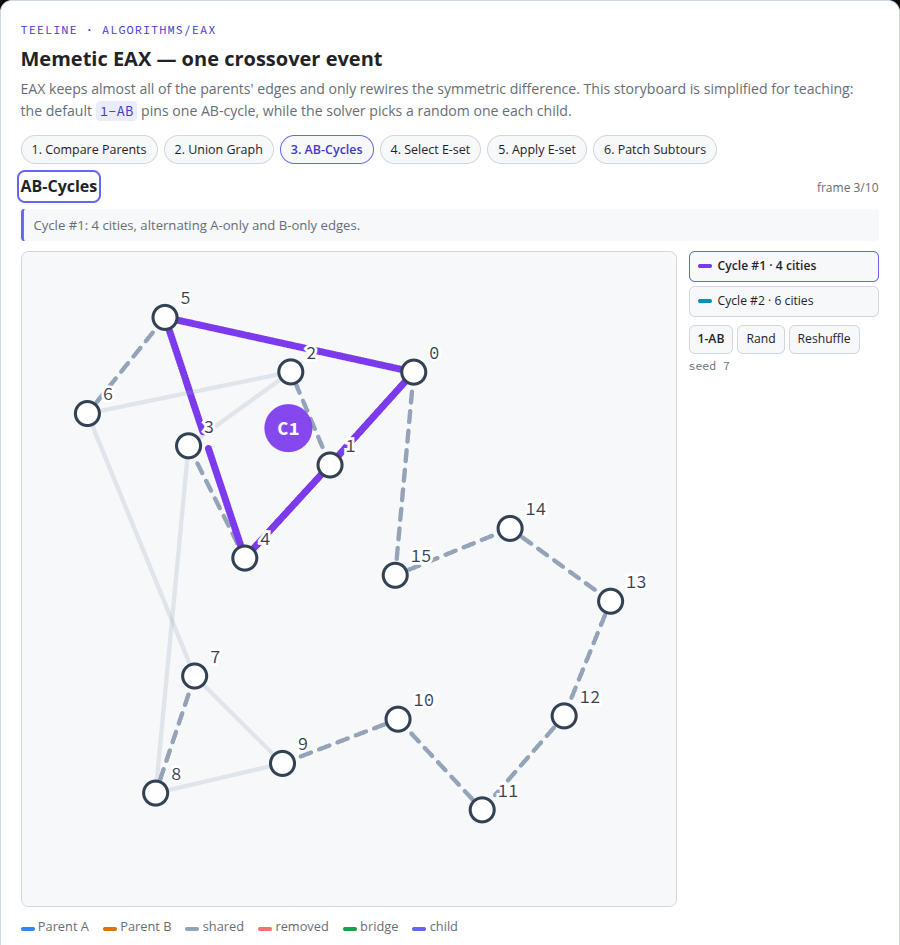
Swap a few loops. Start from a copy of tour A. For each loop you pick, delete its A-roads and put in its B-roads. Every city the loop touches loses one road and gains one, so each city still has exactly two roads — the tour never loses its shape. What it usually loses is being a single loop: the result is several disconnected mini-loops.
Stitch and polish. Patch the mini-loops back into one tour, merging the smallest first and preferring short candidate edges. Here is the real magic of the whole method: the stitch is allowed to use a road that was in neither parent. That is mutation for free, delivered precisely where the crossover broke the tour. A quick 2-opt pass — uncross edges until no simple swap shortens the loop — cleans up the seams. Bolting local search onto every child makes it a memetic algorithm, which gives teeline’s Memetic EAX its name.
Quietly extraordinary — and two catches
The usual currency for a TSP heuristic is gap: how much longer its tour is than the best known one, as a percentage. Zero means it tied the optimum.
On 12 standard TSPLIB benchmark maps, Memetic EAX’s median gap is 0.00% on every single one, over five runs each. The largest map, dsj1000 with 1,000 cities, is the only one where any run missed at all: the worst was 0.04% above optimal, and the median run took about 30 seconds on a desktop CPU. The benchmark allows it 300 seconds.
I did not expect that when I added the solver. I expected an interesting algorithm that was too slow to matter. It is slow. It is also, in the median run, matching the known optimum on every map in the benchmark.
Now the catches, because there are two.
The first is permanent: EAX is a heuristic. A gap of 0.00% means “matched a route someone else proved optimal”, on maps whose optimum is already known. On a brand-new map it will give you a remarkably short tour, not a certificate that no shorter tour exists. That is the honest relationship between EAX and the P vs NP question. Heuristics do not defeat NP-hardness; they route around it for the inputs people actually have.
The second is the price of all that machinery: speed. In the native benchmark, 2-opt finishes berlin52 in about two hundredths of a second; Memetic EAX takes about three seconds. Every child pays for a crossover, a patch, and a local-search polish. On a 52-city map that trade is silly. On a 1,000-city map where every 0.1% matters, it is the whole point: you are buying quality per run, not tours per second.
Try it
The interactive explainer is the best place to see the move — scrub through it once. The algorithm page has the full description, the options, and the benchmark table, with the references at the bottom.
If you would rather feel the gap close, open the solver. It loads berlin52 and its optimal tour, so the gap column is live. Run Nearest Neighbor and note the gap — about 19% on this map. Then choose Memetic EAX from the “All solvers…” menu and watch it land on 0.00%. Give it a minute or two: the browser build is much slower than the native benchmark.
If you have the CLI installed:
teeline solve eax -i berlin52.tspTSP is NP-hard in the worst case. Your map is probably not the worst case.